With the rapid rise of large language models, most of us just build applications that consume third party API, this is so common we even have a word for it, “GPT wrapper”, and honestly, that works fine most of the time. You wire up a model, wrap some code around it, ship it, and everyone’s happy.
And here’s the thing, while we’re all reaching for the same handful of API providers, there’s a tonne of open-source LLMs out there, Llama, Mistral, Qwen, Gemma, and plenty more, just sitting there waiting to be used. Most of us aren’t taking advantage of them at all.
But back to the APIs for a second, because they don’t always cut it.
Every now and then a project comes along that doesn’t quite fit. Maybe a client wants something very custom, and you find out the provider’s model either doesn’t have that capability, or only offers a diluted version of it. So you do what we all do. You start trying things. Prompt engineering, RAG, MCP, tools, all of it. You tweak, you retry, you tweak again.
Sometimes one of these techniques or a combination does the trick and the problem goes away. But sometimes they just don’t work at all, no matter how much you push. You’ve hit a wall.
So what do you do once you hit that kind of road block?
That’s exactly what this series of articles are about. And as you’ll see, those open-source models we just mentioned are about to become very useful. I’ll be posting this articles gradually untill complete, by the time most of you are reading this, it might all be already posted.
Across this series of articles, we’ll cover both the theory behind fine-tuning and the hands-on practice of actually doing it. Here’s what’s coming up:
- RAG vs fine-tuning, and how to know which one your problem actually needs
- The different types of fine-tuning and what sets them apart
- Quantization, both the theory of how it works and how to implement it in practice
- What base models really are, and why they matter
- Fine-tuning a base model from start to finish, with MLOps experiment tracking baked in so you can measure what’s actually happening
Let’s begin by looking at a case study, a fictional one I created.
The Scenario
Imagine you work as an AI engineer at a hospital. Let’s call it Tantanila Hospital. The Head of Technology has been eager to bring AI into the hospital’s products for some time now, and one Monday morning, he calls you into his office with a task.
The hospital wants a chatbot, something patients can use to ask questions about the hospital and its services. But there’s a catch. Two of them, actually.
First, the chatbot needs to speak in a very specific tone, the warm, professional, slightly reassuring voice the hospital uses across every patient touchpoint, from the front desk to the discharge papers. It can’t sound like a generic AI assistant. It needs to sound like Tantanila.
Second, the chatbot needs to know things only the hospital knows. Visiting hours for each ward. Which specialists are on call this week. What documents a new patient needs to bring. How to navigate from the main entrance to radiology. None of this lives on the public internet, it lives in internal policy documents, staff handbooks, and ward-specific guides.
So here you are. How do you actually build this?
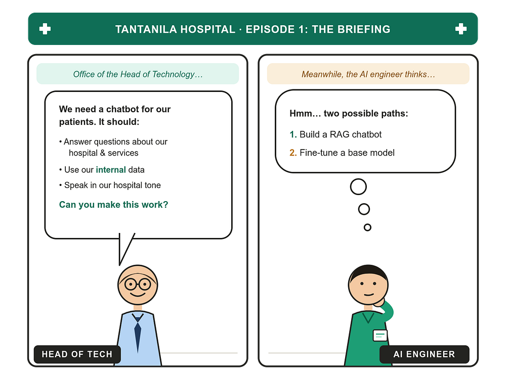
As the Head of Tech finishes laying out the requirements, two paths come to mind. You could build a RAG-based chatbot, or you could fine-tune a base model. Let’s walk through both.
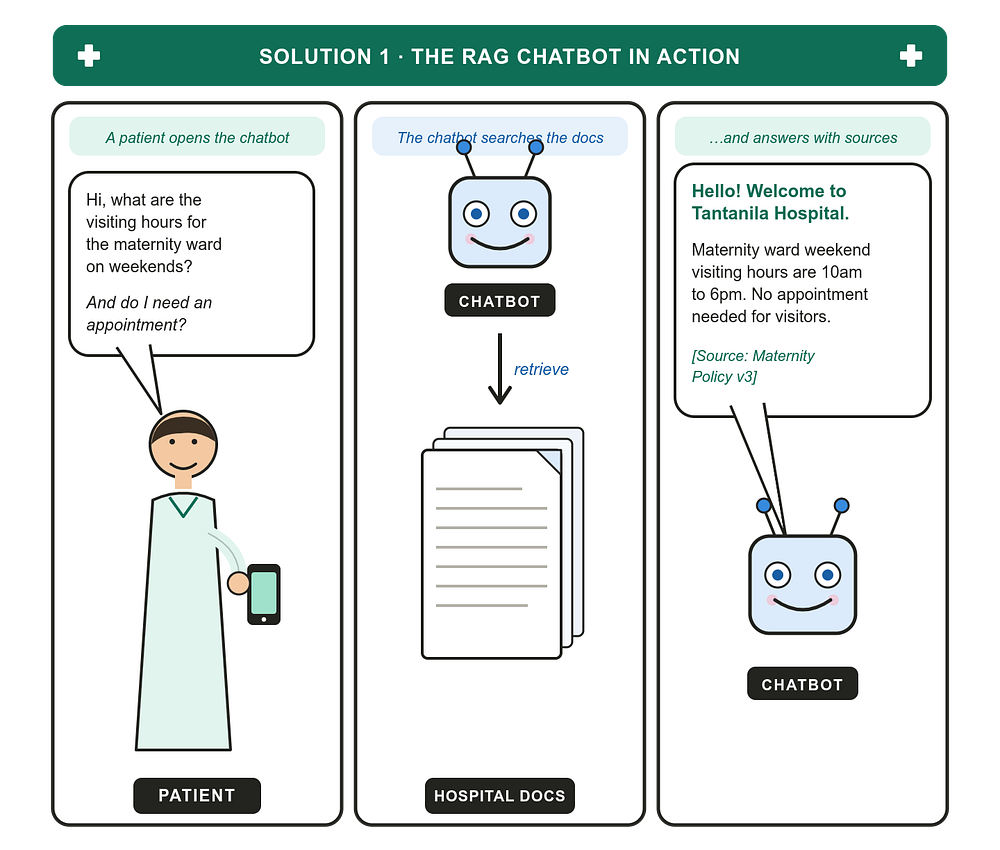
Solution 1: Building a RAG-Based Chatbot
RAG stands for Retrieval-Augmented Generation. The idea is simple, and the name basically tells you what it does: when a patient asks a question, the system first retrieves the most relevant information from the hospital’s documents, then hands those documents to a language model so it can generate an answer grounded in what it just read.
You don’t change the model at all. The model, say, a general-purpose LLM like GPT-4, Claude, or an open-source equivalent, stays exactly as it came out of the box. What you change is what it sees at the moment a patient asks a question, the context you provide it with.
Here’s how the flow works in practice:
- You take every hospital document (policies, ward guides, FAQs, staff handbooks) and chop it into bite-sized chunks.
- You convert each chunk into a vector embedding and store it in a vector database.
- When a patient asks a question, you embed their question too, and pull the chunks whose embeddings are closest to it.
- You stuff those chunks into the prompt along with the question, and let the model answer.
Why RAG fits this problem well
The hospital’s information changes. New wards open. Visiting policies get updated. A doctor’s schedule shifts. With RAG, you don’t retrain anything when this happens, you just update the documents in the vector store, and the chatbot’s answers update automatically the next time someone asks.
It’s also auditable. When the chatbot says “maternity ward weekend hours are 10am to 6pm,” it can cite the exact policy document and version it pulled that from. In a hospital setting, where being able to point to the source of an answer is genuinely important, this is a big deal.
And it’s cheap to start. You’re not paying for GPU time to train anything. You pay for embedding API calls, vector storage, and inference, all of which are well-understood, predictable costs.
Where RAG struggles
The tone problem doesn’t fully go away. You can put instructions in the system prompt , “respond in a warm, professional tone, like a Tantanila Hospital receptionist would” and a strong base model will do a decent job of following that. But it won’t be perfect. The model’s underlying personality leaks through, especially on edge cases, long conversations, or unusual questions. You’ll find yourself constantly tweaking the system prompt to nudge the tone back where you want it.
RAG also depends entirely on retrieval quality. If your chunks are too small, you lose context. If they’re too big, you waste tokens and the model gets distracted. If the patient phrases their question in a way that doesn’t match how the documents are written, retrieval misses the relevant chunk and the model has to either guess or admit it doesn’t know.
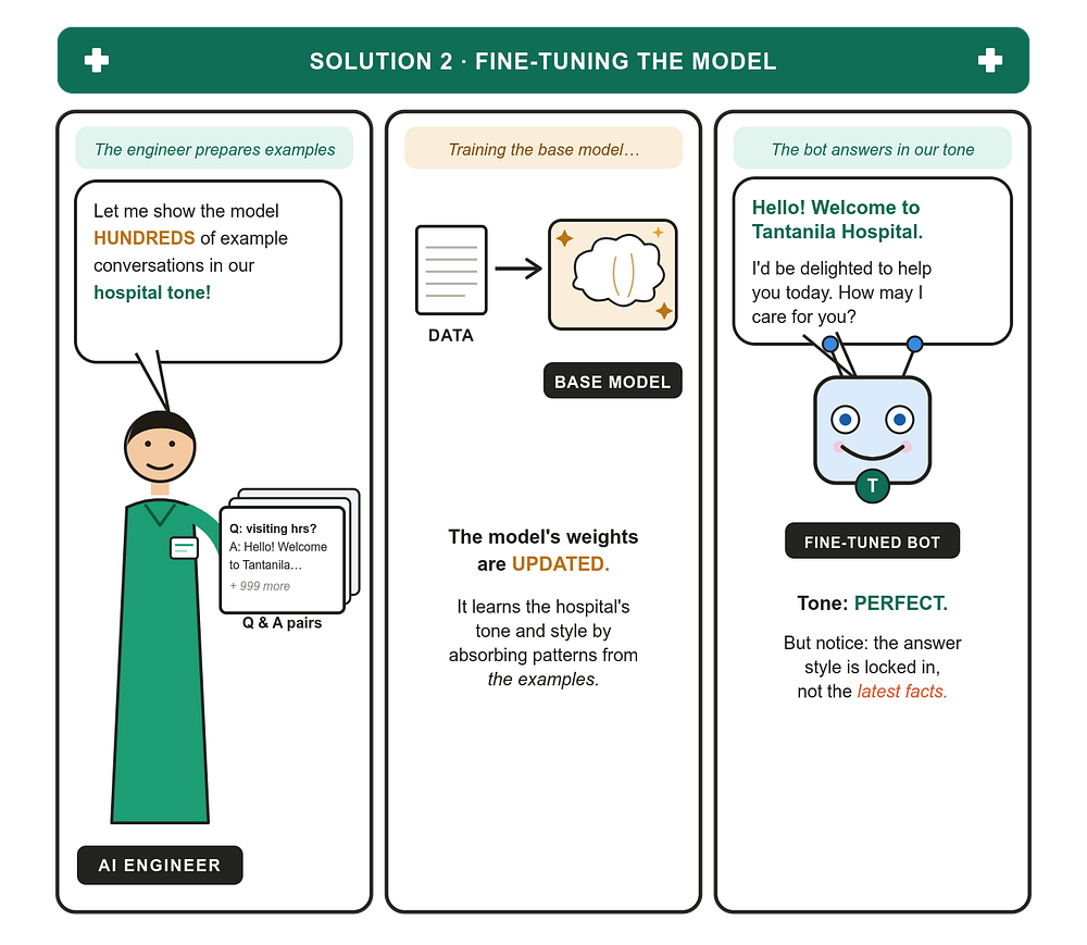
Solution 2: Fine-Tuning a Base Model
Fine-tuning takes a completely different approach. Instead of giving the model external documents to read at runtime, you teach the model itself what Tantanila Hospital sounds like and what it knows.
You start with a pre-trained base model, one that already understands English, conversation, and the world in general. Then you continue training it, but only on examples specific to your problem: hundreds (sometimes thousands) of Q&A pairs that show the model exactly how a Tantanila chatbot should respond.
Each training example looks something like:
Patient: What are the visiting hours for the maternity ward on weekends? Tantanila Chatbot: Hello! Welcome to Tantanila Hospital. I’d be delighted to help. Our maternity ward welcomes visitors on weekends from 10am to 6pm, and no appointment is needed.
Show the model enough of these, and its internal weights gradually shift to produce that exact style on its own. The tone, the greeting, the phrasing, it all becomes baked in.
Why fine-tuning fits this problem well
For tone, fine-tuning is unmatched. A fine-tuned model doesn’t follow tone instructions,it is the tone! There’s no prompt fragility, no drift over long conversations, no awkward edge cases where the model suddenly sounds like a generic chatbot. Every response carries the Tantanila voice because the model has been reshaped to produce that voice.
It can also be faster at inference, because you’re not stuffing the prompt full of retrieved documents on every turn. The model already “knows” the things you taught it, so the prompt stays small.
Where fine-tuning struggles
The hospital’s facts are exactly what you don’t want to bake into the model. Once the model has learned that “maternity weekend hours are 10am to 6pm,” changing that fact means going back, building new training examples, and running another fine-tuning job. That’s slow, expensive, and risky, you might accidentally degrade other things the model used to do well.
Fine-tuning is also opaque. When the model answers, you can’t point to a specific document it consulted. The knowledge is now spread across billions of parameters, which is great for fluency and terrible for auditability.
And it requires good data. Hundreds or thousands of carefully written, consistent Q&A pairs. If your examples have inconsistent tone, contradictory facts, or weird formatting, the model will dutifully learn those problems too.
So Which One Should You Pick?
The honest answer for Tantanila Hospital is: probably both, but starting with RAG.
The hospital’s facts, visiting hours, ward locations, specialist schedules, policies, these are exactly the kind of thing that benefits from retrieval. They change, they need to be auditable, and they live in documents you already have. RAG handles all of this naturally.
The hospital’s tone is what benefits from fine-tuning. But you don’t need to fine-tune just to get a decent tone out of a strong base model. A well-crafted system prompt and a few in-context examples will get you most of the way there. Fine-tuning becomes worth the investment when you’ve outgrown that, when you have enough real patient conversations to learn from, and when consistent voice has become a genuine product differentiator rather than a nice-to-have.
A useful rule of thumb:
- RAG is for what the model needs to know.
- Fine-tuning is for how the model needs to behave.
For Tantanila, that means RAG today, fine-tuning tomorrow, and quite possibly both running together, with the fine-tuned model handling the voice while RAG handles the facts.
NOTE:
Before you even begin fine tuning a model, know it costs alot of investment, financially and time wise.
Make sure you have exusted all other techniques like prompt engineering, RAG, MCP, tools, context engineering etc before venturing into fine-tuning.
Types of Fine-Tuning
So you’ve decided fine-tuning is part of the answer. But “fine-tuning” isn’t one technique, it’s a family of them, and which one you pick has big consequences for cost, training time, and how many GPUs you need to keep alive at 3am.
Broadly, there are two camps:
- Full fine-tuning
- Parameter-Efficient Fine-Tuning (PEFT), the most popular flavours being LoRA and QLoRA
Full Fine-Tuning
Full fine-tuning is the original approach: take every weight in the base model, and update every single one of them during training. If the model has 7 billion parameters, you’re training all 7 billion.
This gives you the most flexibility, the model can change in any direction the data pulls it, but it’s brutally expensive. You need enough GPU memory to hold the model’s weights, their gradients, and the optimizer state (which for Adam is roughly 2× the model size on its own). For a 7B model, that’s easily 60+ GB of VRAM before you’ve even loaded a batch of training data. For a 70B model, it’s a small cluster.
You also end up with a full copy of the model for every task you fine-tune on. Fine-tuned the chatbot for Tantanila? That’s a 14GB file. Fine-tuned another one for a different hospital? Another 14GB. Stack up a few of these and your storage costs start hurting.
Parameter-Efficient Fine-Tuning (PEFT)
PEFT is the response to all of this. The core idea: don’t change the original model at all, instead, train a small number of new parameters that sit alongside the model and influence its behaviour.
The two PEFT techniques you’ll hear about most are LoRA and QLoRA. QLoRA is essentially LoRA with the base model quantised (compressed) to 4-bit precision to save memory, so let’s focus on LoRA itself.
LoRA (Low-Rank Adaptation)
LoRA targets specific weight matrices inside the transformer, typically the attention projection matrices: W_q, W_k, W_v, and W_o. Call any one of these W.
In normal fine-tuning, you’d update W directly. In LoRA, you do something more clever:
Keep
Wfrozen. Define a new matrixW' = W + ∆W, and during training, only ever update∆W.
Which raises a perfectly reasonable question, the one I bet just popped into your head:
If LoRA is supposed to be parameter-efficient, doesn’t adding a brand new ∆W matrix mean you now have more parameters, not fewer?
You’re absolutely right that adding ∆W naively would increase the parameter count. If W is a 4096×4096 matrix and ∆W is also 4096×4096, you’ve now got twice as many parameters, not fewer. That would be a terrible deal.
The trick, and the entire reason LoRA works, is in how ∆W is stored.

LoRA never stores ∆W as a full matrix. Instead, it decomposes it into two much smaller matrices:
∆W = B × A
Where:
Bhas shaped × rAhas shaper × dris the rank, a small number, typically 4, 8, 16, or 32
When you multiply B × A, you get a d × d matrix that’s the same shape as ∆W would have been, but you only ever stored and trained the small B and A matrices. The full ∆W is conceptual; it’s reconstructed on the fly when needed.
Run the numbers for a single attention matrix in a typical transformer:
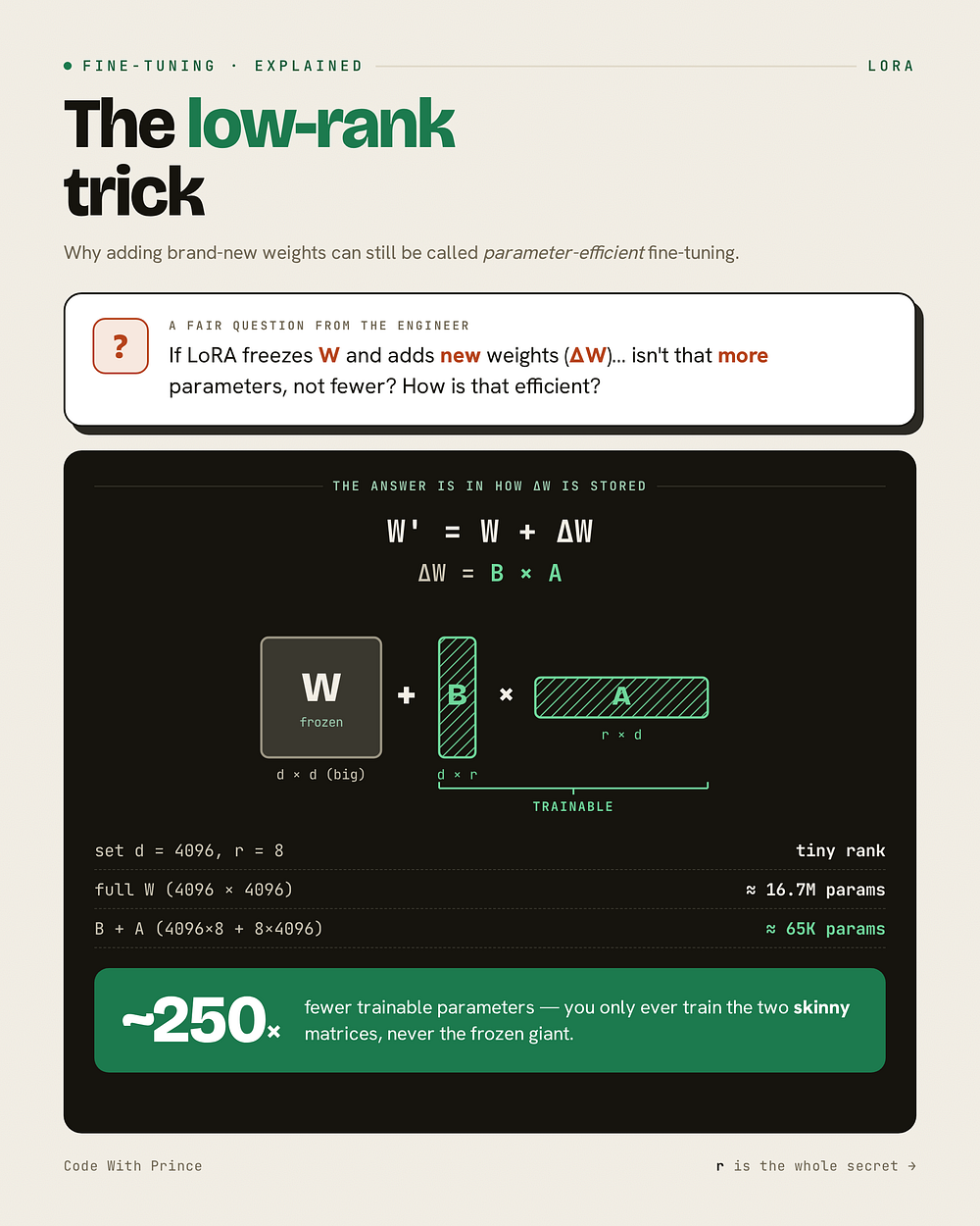
That’s the parameter efficiency. You’re not really adding parameters in any meaningful sense, you’re adding a tiny set of trainable parameters that, through matrix multiplication, can express updates to a much larger frozen matrix.
The bet LoRA is making, and the bet that turns out to work surprisingly well in practice, is that the update you need to apply to W for a specific task is intrinsically low-rank. You’re not teaching the model fundamentally new capabilities; you’re nudging existing ones in a particular direction. And those kinds of nudges, it turns out, don’t need millions of parameters to express. They need a few thousand.
QLoRA (Quantized Low-Rank Adaptor)
LoRA already saved us a huge number of trainable parameters, but there’s still one big cost we haven’t touched, the base model itself. Even though we freeze it, we still have to load it into GPU memory to run the forward and backward passes through it. For a 7B model in standard precision, that’s around 14 GB of VRAM just sitting there, untouched, while we train our tiny adapters. For a 70B model, it’s 140 GB, which is well beyond what a single consumer GPU can hold.
QLoRA’s contribution is to attack that base model memory cost head-on, by quantizing the frozen base model down to 4-bit precision before LoRA ever touches it.
What is Quantization?
Quantization is the process of representing the same numbers using fewer bits. In a neural network, every parameter is just a number, and how many bits we use to store that number directly determines how much memory the model consumes.
Take the original GPT-2 model, with 124 million parameters. By default, each parameter is stored as a float32, which uses 4 bytes per number (32 bits ÷ 8 = 4 bytes)(1 byte = 8 bits).
124,000,000 params × 4 bytes = 496,000,000 bytes ≈ 0.496 GB
So GPT-2 takes about half a gigabyte just to hold the weights at float32.
Now imagine we could represent each parameter using float16 instead (2 bytes per number):
124,000,000 params × 2 bytes = 248,000,000 bytes ≈ 0.248 GB
We just halved the memory footprint, without changing the model architecture or retraining anything. We only changed how each number is stored. The scaling matters more on bigger models, on a 70B model, going from float32 to float16 saves about 140 GB of GPU memory.
Float32, Float16, Int8, Int4
Let’s get specific about what each of these formats actually is.
Float32 (FP32) uses 32 bits per number, split into 1 sign bit, 8 exponent bits, and 23 mantissa bits. It can represent a huge range of values with high precision, roughly from 10^-38 to 1⁰³⁸, with about 7 decimal digits of accuracy. This is the default for training, because gradient updates can be very small, and you want to preserve them faithfully.
Float16 (FP16) uses 16 bits, 1 sign bit, 5 exponent bits, and 10 mantissa bits. Smaller range, less precision, but still a continuous floating-point number.
Int8 is a different beast. It’s not floating-point at all, it’s an 8-bit integer, which means it can only represent 256 distinct values (from -128 to 127). No fractional values, no exponents, just integers.
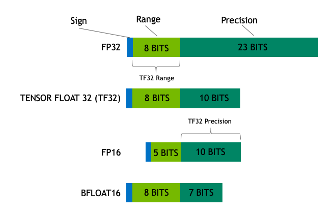
Int4 is even more restrictive, only 16 distinct values (from -8 to 7).
The obvious question, how do you represent a continuous-valued weight like 0.0234 using a value that can only be an integer between -8 and 7?
How Quantization Actually Works
The trick is a thing called a scale factor. Quantization stores two things, the integer value, and a scale that tells you how to convert back to a real number.
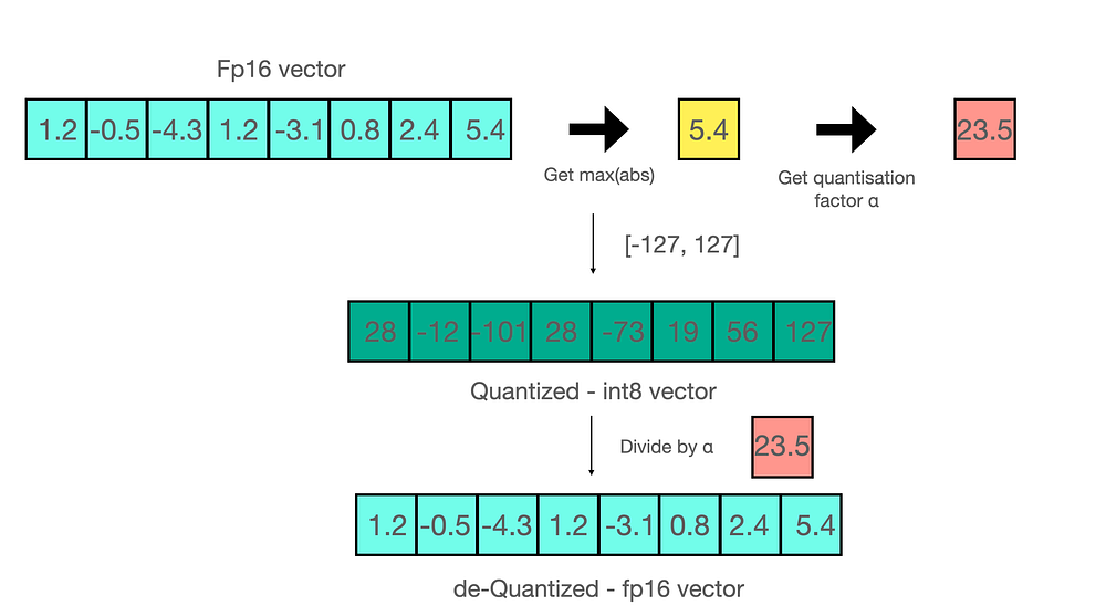
Suppose we have a group of float32 weights and we want to quantize them to int8:
weights = [0.12, -0.45, 0.78, -0.23, 0.05, -0.91, 0.34]
Step 1, find the absolute maximum:
abs_max = 0.91
Step 2, compute the scale. Int8 ranges from -127 to 127 (we use 127, not 128, to keep things symmetric):
scale = abs_max / 127 = 0.91 / 127 ≈ 0.00717
Step 3, quantize each value by dividing by the scale and rounding to the nearest integer:
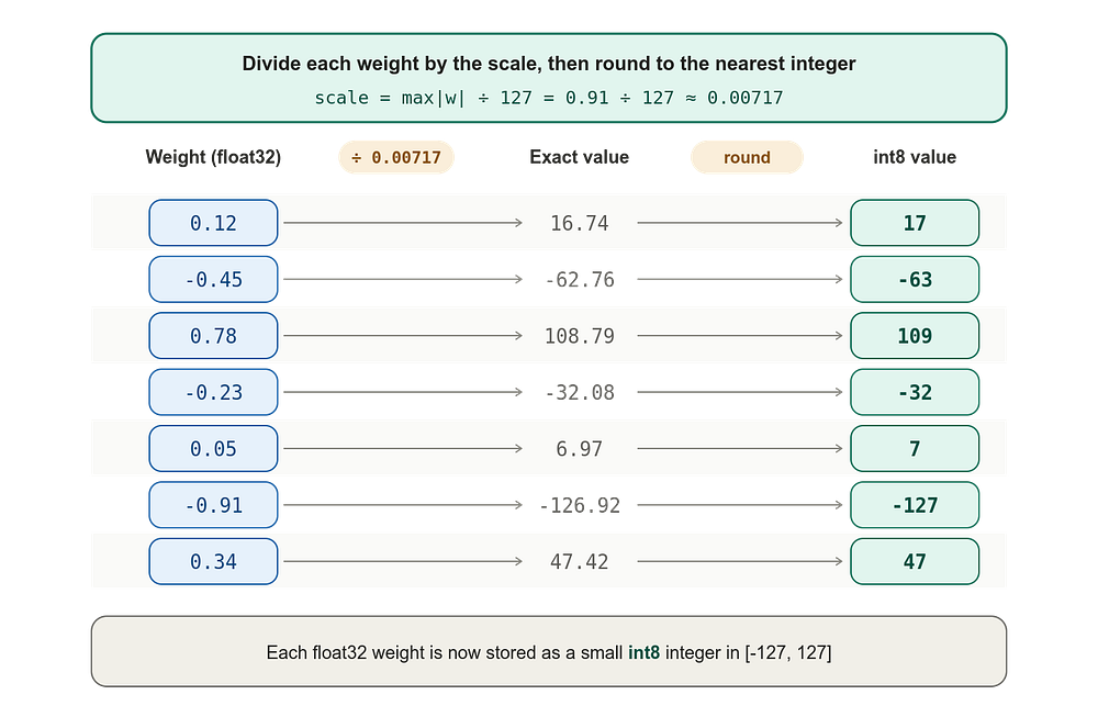
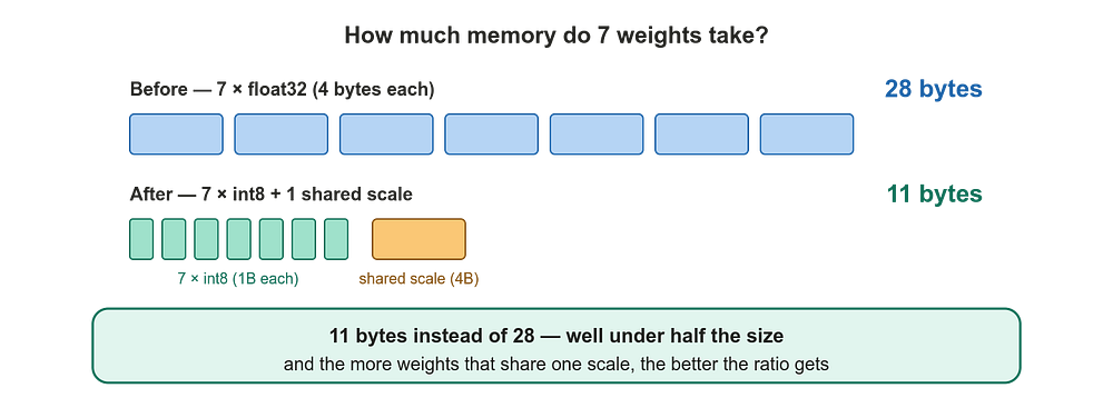
Now instead of storing seven float32 values (28 bytes), we store seven int8 values (7 bytes) plus one float32 scale (4 bytes), for a total of 11 bytes. We’ve nearly cut memory usage by a third, and the larger the group of weights sharing one scale, the better that ratio gets.
To dequantize (turn the integers back into approximate floats), you just multiply by the scale:
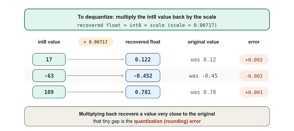
The reconstructed values aren’t exactly the originals, there’s a small rounding error, but they’re close enough that the model still works.
For a FP16 to int8 quantization:
For more reading: LLM.int8(): zero degradation matrix multiplication for Large Language Models
NF4 (4-bit NormalFloat)
Standard int4 quantization assumes weights are spread out uniformly across their range, but in real neural networks they aren’t. Weights tend to follow a roughly normal distribution, most of them are clustered around zero, with progressively fewer weights at the extremes.
NF4, which stands for 4-bit NormalFloat, is a quantization format designed specifically for this. Instead of spacing the 16 representable values uniformly between the minimum and maximum, NF4 spaces them so that more of them sit near zero where most weights live, and fewer sit out at the tails where weights are rare.
The result, the same 4 bits per weight, but a much better fit for what neural network weights actually look like, so the rounding error is lower and model quality holds up better than with naive int4. NF4 was introduced in the original QLoRA paper, and it’s the default 4-bit format used in QLoRA today.
Double Quantization
Here’s a clever follow-up. We just saw that quantization requires storing scale factors alongside the integer weights. But those scales are themselves float32 numbers, and if we have one scale per small group of weights (say one scale per 64 weights, which is standard), the scales start to add up.
For a 7B model, that’s about 110 million scale factors, which works out to roughly 440 MB just for the scales. Not nothing.
Double quantization is the obvious next move, quantize the scales too. Take the float32 scales, group them, compute a scale-of-scales, and store the scales themselves as smaller numbers (typically 8-bit).
It’s the same idea as zipping a file that’s already been zipped. You’re compressing the metadata of the compression itself. Done right, it saves an extra 0.4 to 0.5 bits per parameter, which on a 70B model is multiple gigabytes of GPU memory.
This notebook is a hands-on companion to everything we just covered on quantization. It loads the same model three different ways using Hugging Face Transformers and bitsandbytes: the full-precision Llama 3.2 1B base model, an INT8 version (load_in_8bit), and a 4-bit NF4 version with double quantization and a bfloat16 compute dtype, which is the exact recipe QLoRA uses. So instead of just reading about FP32 vs INT8 vs NF4, you get to load all three side by side and poke at them yourself.
From there it runs a few comparisons to make the trade-offs concrete. It prints the memory footprint of each model (the base sits around 4.9 GB, INT8 drops to about 1.7 GB, and 4-bit comes in near 1.2 GB), then pulls the raw weights from the first attention layer of each model so you can actually see the difference between full-precision floats and their quantized forms. After that it generates text from all three models on the same prompt to eyeball whether quality holds up, and finally it calculates perplexity (both on a small sample and on a slice of WikiText-2) so there’s a real number measuring how much, if anything, you lose by quantizing.
One thing to note: I used MLflow to log and track these experiments, so the last few cells log each variant’s quantization params, memory footprint, perplexity scores, and even the generated text as an artifact. If you want that same tracking, you’ll need to point the notebook at your own MLflow server (set your tracking URI and credentials). If you don’t care about tracking, you can safely skip those cells, everything else in the notebook runs fine without them. The full notebook is attached below.
Google Colab
Edit descriptioncolab.research.google.com
Three Use Cases of Quantization
Beyond shrinking model files, quantization is useful for:
- Inference on smaller hardware. A quantized 7B model can run on a single laptop GPU, sometimes even on CPU. The unquantized version cannot.
- Fitting bigger models into the same GPU. A 70B model in float16 needs around 140 GB, far beyond a single H100. The same model in 4-bit fits in about 35 GB, which one H100 can hold comfortably.
- Faster inference. Smaller numbers move faster through memory, and on modern GPUs, certain quantized operations are accelerated in hardware. You often get a real wall-clock speedup, not just a memory saving.
So What Is QLoRA?
QLoRA combines all of these ideas into one technique. The recipe:
- Take the base model and quantize it to 4-bit NF4, freezing it permanently in that compressed form.
- Apply double quantization to the scale factors, squeezing out the extra overhead.
- Run LoRA on top, training only the tiny B and A adapter matrices, exactly as before.
- Use paged optimizers (more on this in a moment) to handle GPU memory spikes during training.
The frozen base model sits in 4-bit NF4 the entire time. When the forward pass needs to use a weight, it gets dequantized on the fly to a higher precision (usually bfloat16), multiplied with whatever it needs to multiply with, and then thrown away. The 4-bit version is the only version that’s permanently stored.
The LoRA adapters themselves stay in full precision, because they’re tiny and we want the actual training updates to be as accurate as possible.
The combined effect is dramatic. A 65B model that would normally need a multi-GPU server to fine-tune, even with LoRA, can be fine-tuned on a single 48 GB GPU with QLoRA. That’s the headline result from the original paper.
Paged Optimizers
There’s one last piece, paged optimizers.
When you train a model, the optimizer (usually AdamW) maintains internal state for every trainable parameter, momentum and variance estimates. This state is typically twice the size of the trainable parameters themselves. Even with LoRA, where only the adapter weights are trainable, you can still hit memory spikes during training, especially when processing long sequences or large batches.
If those spikes push you past the GPU’s memory limit, training crashes. Out of memory, retry, lose hours of progress.
Paged optimizers solve this by borrowing an idea from operating systems, paging. When the GPU runs low on memory, some of the optimizer state gets automatically moved out to CPU RAM, freeing up GPU memory for whatever is in the hot path. When that paged-out state is needed again, it’s swept back to GPU memory transparently.
It’s slower than keeping everything on GPU, but slower is better than crashed. In practice, paging only kicks in during the brief memory spikes, so the average training speed is barely affected.
Together, 4-bit NF4 quantization, double quantization, LoRA adapters, and paged optimizers form the four ingredients of QLoRA, and they’re what makes fine-tuning large models on consumer hardware genuinely possible today.
Why this matters for Tantanila
For a hospital chatbot project, this is the difference between needing a dedicated GPU server and being able to fine-tune on a single consumer GPU overnight. It’s also the difference between shipping one giant model and being able to swap in different LoRA adapters for different departments, one for paediatrics, one for cardiology, one for the emergency desk, each one a few megabytes instead of a few gigabytes, all sharing the same frozen base model underneath.
That’s the real reason LoRA earned its place in the toolbox.
Pre-trained language models are remarkable generalists. They’ve read more text than any human ever could, and they can hold a passable conversation about almost anything. But “passable” is rarely good enough when you have a specific job to do answering medical questions, drafting legal summaries, classifying support tickets, or generating code in your team’s internal style. For that, you need to teach the model what your problem actually looks like. That’s fine-tuning.
Conclusion
Congratulations for making it this far! We’ve covered a lot of ground. We started with a simple problem at Tantanila Hospital and used it to figure out when to reach for RAG versus fine-tuning, then went deep into what fine-tuning actually is: full fine-tuning, PEFT, and the clever low-rank trick behind LoRA that lets you train a tiny fraction of the parameters. From there we unpacked QLoRA piece by piece, which led us into quantization, the art of squeezing floats down into smaller integers, and we even loaded a model in three different precisions to measure what each one really costs.
The thread running through all of it is the same: these techniques exist to make working with large models practical on hardware you actually have, without giving up much of what makes the models good. RAG, LoRA, quantization, they’re all different answers to the same question of how to get the behaviour you need without the price tag you can’t afford.
In the next article we’ll shift from theory to play. We’ll load base models in Google Colab, tinker around with them directly, and get a real feel for how they behave before any fine-tuning happens. Along the way we’ll answer a question that’s easy to gloss over but matters a lot: what actually is a base model, and how is it different from the polished, instruction-following models you’re used to talking to? Once that clicks, fine-tuning will make a whole lot more sense. See you in the next one.
Other platforms where you can reach out to me:
Happy coding! And see you next time, the world keeps spinning.